Categories
Uncategorized

Uploading

TN Result Data base is Uploading Try After some time


Automobile insurance

Comparing automobile insurance quotes can facilitate purchasers purchase a regular low price motorcar insurance. Since the contract is signed, even just in case of Associate in Nursing depression, drivers won’t got to pay additional for his or her coverage. buying automobile insurance will currently be done on-line

Here, purchasers will review multiple plans in barely some minutes. The brokerage service is free and therefore the web site uses an expert computer program to assist purchasers notice the correct plans for his or her vehicles. during this means, drivers now not got to decision numerous agents or visit multiple websites.

In order to shop for Associate in Nursing advantageous coverage policy, purchasers ought to initial choose a budget. this can offer them a tenet once buying coverage. Then, they must decide what proportion coverage they require. it’s additionally necessary to notice that bound styles of automobile insurance plans offer coverage just for bound things.

Automobile insurance premiums

Knowing these necessary things before comparison motorcar insurance quotes can facilitate drivers select a coverage arrange that’s right for his or her vehicle. automobile insurance premiums are influenced by the sort of automotive that somebody drivers and by the client’s driving record. By comparison numerous automobile insurance quotes, drivers are able to scale back their coverage expenses by over V-day.

The skilled computer program permits drivers to customise their searches. they’ll select what proportion coverage they have and what form of automobile insurance they require. the web site can displays plans that ar relevant for every driver.

“In order to search out an inexpensive and advantageous automobile insurance arrange, drivers ought to compare multiple quotes. this will currently be done on one web site, in an exceedingly straightforward and convenient means.” same Russell Rabichev, selling Director of web selling Company.

There is a web supplier of life, home, health, and motorcar insurance quotes.

Why ICICI Lombard is the smart choice to secure yourself and the things you love

During FY2017, we settled 99.4 % health insurance claims and 92.2% motor insurance claims (own damage) within 30 days of claim filing.

Why Bajaj Allianz General Insurance

Surprises are an inevitable part of life – good and bad. But why deal with unpleasant surprises when you have insurance? General insurance will help you mitigate the financial losses incurred due to damage to the assets you value most. It offers you financial protection against perils faced with regards to your property, vehicle, personal accidents, health and travel. The right general insurance policy will provide you with the right protection against risks or disasters, no matter how big or small.

Why Royal Sundaram Car Insurance Policy?

Royal Sundaram is a company that is dedicated to providing you with the best there is in terms of Insurance Cover. Our Car Insurance Policy is one that not only helps you protect your vehicle but is also cash saving in nature.

Categories
Uncategorized

TamilNadu 12th Result 2018 TN HSC +2 Examination Results

TamilNadu 12th Result 2018 TN HSC +2 Examination Results

TamilNadu 12th Result 2018 TN 12th std result 2018. Tamil Nadu Students of 12th Standard can check their 12th result 2018 in this page. The DSE (Directorate of Secondary Education) of Tamil Nadu will publish the 12th std result 2018.

Tamil Nadu Higher Secondary Result 2018 will be published on May 16 of 2018.

The TN result for HSC will be published as soon as the Tamil Nadu Board release the result 2018.

TamilNadu 12th Result 2018 Date is confirmed and the count down has begin

TamilNadu 12th Result 2018:

The +2 Students are stressed because the results will published by 16th of  this month. From previous year the government of Tamil Nadu has decided not to release the rank of the students which will be continued this year (2018) too.

This is mainly done to reduce the stress of the student to score 1st 2nd 3rd Ranks in the Tamil Nadu public exam.

This process is well received by major percentage of the students. According to them this will retrieve the mental pressure by parents on them.

Few students how score high ranks are disappointed by this act of the Tamil Nadu Directorate of Secondary Education.

TamilNadu 12th Result Statics:

As per Last yesr record  8,93,262 students wrote the exam and 8,22,838 cleared the exam.

TamilNadu 12th Result 2018 TN HSC +2 Examination Results


1,123 Students got centum in Chemistry


3,361 Students got centum in Physics


3,656 Students got centum in Mathematics


221 Students got centum in Biology


8,301 Students got centum in commerce


5,597 Students got centum in accountancy


2,551 Students got centum in business mathematics


Virudhunagar District got pass percentage of 97.85%


Categories
Uncategorized

FLOOD ROUTING

FLOOD ROUTING

FLOOD ROUTING – The stage and discharge hydrographs represent the passage of waves of river depth and discharge respectively.

As this wave moves down the river, the shape of the wave gets modified due to various factors, such as channel storage, resistance, lateral addition or withdrawal of flows, etc.

When a flood wave passes through a reservoir, its peak is attenuated and the time base is enlarged due to the effect of storage.

Flood waves passing down a river have their peaks attenuated due to friction if there is no lateral inflow.

The addition of lateral inflows can cause a reduction of attenuation or even amplification of a flood wave.

Flood routing is the technique of determining the flood hydrograph at a section of a river by utilizing the data of flood flow at one or more upstream sections.

The hydrologic analysis of problems such as flood forecasting, flood protection, reservoir design  and spill design  invariably include  flood routing.

In these applications  two broad categories of routing can be recognised.

These are:

Reservoir routing

Channel routing

In reservoir routing the effect of a flood wave entering a reservoir is studied. Knowing the  volume — elevation  characteristic  of  the  reservoir  and  the  outflow — elevation relationship for the spillways and other outlet structures in the reservoir, the effect of a flood wave entering the reservoir is studied to predict the! variations of reservoir elevation and outflow discharge with time.

This form of reservoir routing is essential (i) in the design of the capacity of spill and other) reservoir outlet structures and (ii) in the location and sizing of the capacity of reservoirs to meet specific requirements.

In channel routing  the change  in the  shape  of a hydrograph  as it travels  down a channel is studied.

By considering a channel reach and an input hydrograph at the upstream end, this form of routing aims to predict the flood hydrograph at various

sections of the reach. Information on the flood-peak attenuation and the duration of levels obtained by channel routing is of utmost importance in ‘ operations and flood- protection works.

A variety of routing methods are available and they can be broadly classified into two categories as: (i) hydrologic routing and (ii) hydraulic routing. 0 methods employ essentially the equation of continuity.

Hydraulic methods, on the other hand, employ the continuity equation  together with the equation of motion of unsteady flow-

The basic  differential  equations  used  in  the  hydraulic  routing,  known  as  St.Venant equations afford a better description of flow than hydrologic methods.

HYDROLOGICAL STORAGE ROUTING (LEVELPOOL ROUTING)

A flood wave 1(t) enters a reservoir Provided with an outlet such as a spill Way T outflow is a function of the reservoir elevation only, i.e. Q =Q (h).

The Storage in the reservoir is a function of the reservoir elevation s = s(h)
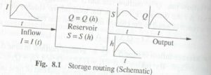
FLOOD-ROUTING HYDROLOGICAL STORAGE ROUTING

Further, due to the Passage of the flood wave through the reservoir, the water level in the reservoir changing with time h =h (t) and hence the storage and discharge change with time required to find the variation of s, h and Q with time.

where H = head over the spill way, L= effective length of the Spill way crest and C = coefficient of discharge .

Similarly for other forms of outlets such as gated Spill ways sluice gates, etc. other relations for Q (h) will be available,

For reservoir routing, the following data have to be known:

1. Storage volume vs elevation for the reservoir:

2. Water surface  elevation  vs  outflow  and  hence  storage    outflow discharge;

3 inflow hydrograph I = I(t and

4. Initial values of S,/and Q at time: =0

There are a V of methods available for routing of floods through a reservoir. All of them  use but in various  re arranged  manners.

As the  horizontal  surface  is assumed in the reservoir, the storage routing is also known as leve1 pool routing.

HYDRAULIC METHOD FOR FLOOD ROUTING

Only for highly simplified eases can one obtain the analytical solution of these equations. The development of modern, high-speed digital computers during the past two decades has given rise to the evolution of many indicated  numerical techniques.

The  various  numerical  methods  for  solving  St.venant  equations  can  be  broadly classified into two categories:

Approximate Methods

Complete Numerical methods

These methods are based on the equation of continuity only or on a drastically curtailed equation of motion.

The hydrological method of storage routing and Muskingum channel routing belong to this category. Other methods in this category are diffusion analogy and kinematic wave models.

Complete Numerical Methods

These are the essence of the hydraulic method of routing and are classified into many categories as below:

In the direct method, the partial derivatives are replaced by finite differences and the resulting algebraic equations are then solved. In the method of characteristics (MOC)

St Venant equations are converted into a pair of ordinary differential equations (i.e. characteristic  forms) and  then  solved  by finite  difference  techniques.

In the  finite element method (FEM) the system is divided into a number of elements and partial differential equations are integrated at the nodal points of the elements.

The numerical schemes are further classified into explicit and implicit methods.

In the explicit method the algebraic equations are linear and the dependent variables are extracted explicitly at the end of each time step.

In the implicit method the dependent Variables occur implicitly and the equations are nonlinear. Each of these two methods have a host of finite- differentiating schemes to choose from.

ROUTING IN CONCEPTUAL HYDROGRAPH DEVELOPMENT

Even though the routing of floods through a reservoir or channel discuss previous section  were  developed  for  field  use,  they  have  found  another  important  in  the conceptual studies of hydrographs.

The FLOOD ROUTING through a reservoir attenuation and channel  routing  which  gives translation  to an input hydrograph  are treated as two basic modifying operators.

The following two fictitious intensities in the studies for development of synthetic hydrographs through conceptual models.

1. Linear  reservoir:  a  reservoir  in  which  the  storage  is  directly  proportional  to discharge, (S = KQ). This element is used to provide attenuation to flood wave.

2. Linear channel: a fictitious channel  in which  the  time  required  to discharge  Q through a given reach is constant. An inflow hydrograph pass through such a channel with only translation and no attenuation.

Conceptual modelling for Hill development has undergone rapid progress Since the first work by Zoch (1937). Detailed reviews of various contributions to this field are available in Refs 2 and 3 and the details are beyond the scope of this book However, a

simple method, viz, Clark’ s method (1945) which utilizes the Muskingum method of routing through a linear reservoir is indicated below as a typical example of the use of routing in conceptual models.


Routing

The linear reservoir at the outlet is assumed to be described by S = KQ, where K is the storage time constant. The value of K can be estimated by considering the point of inflection P of a surface runoff hydrograph .

At this point the inflow into the channel has ceased and beyond  this point  the flow is entirely due to withdrawal  from the channel storage, The continuity equation
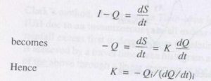
Routing

where suffix i refers to the point of inflection, and K can be estimated from a known surface runoff hydrograph of the catchment

The constant K can also he estimated from the data on the recession limb of a hydrograph.

Knowing K of the linear reservoir, the inflows at various times are routed by the Muskingum  method.

Note  that  since  a  linear  reservoir  is used  .  The  inflow  rate between an inter-isochrone area A, km with a time interval   t (h) is Routing  of the time-area histogram by the above equation gives the ordinates of IUH for the catchment.

Using this IUH- any other D-h unit hydrograph can be derived.

Other links:

HYDROLOGIC CYCLE
PRECIPITATION
RAIN GAUGE
EVAPORATION
INFILTRATION
GROUNDWATER
Water Table
AQUIFER PROPERTIES
DARCY’S LAW
FLOOD FREQUENCY STUDIES
RECURRENCE INTERVAL
GUMBEL’S METHOD

Categories
Uncategorized

GUMBEL’S METHOD

GUMBEL’S METHOD

This extreme value distribution was introduced by Gumbel (1941) and is commonly  known as gumbel’s  distribution.

It  is  one  of  the  most  widely  used probability-distribution  functions for extreme values in hydrologic and meteorologic studies for  prediction of flood peaks, maximum rainfalls, maximum wind speed, etc.

Gumbel defined  a flood as the largest of the 365 daily flows and the annual series  flood  flows constitute  a series of largest  values  of flows.

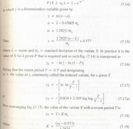
According  to his theory extreme events, the probability of occurrence of an event equal to or larger than a value x0 is

Since the practical annual data series of extreme events such as floods., maximum rainfall depths etc., all have finite lengths of record, Eq. (7.19) is modified to account for finiite N as given below for practical use.

GUMBEL’S METHOD

Gumbel Probability Paper

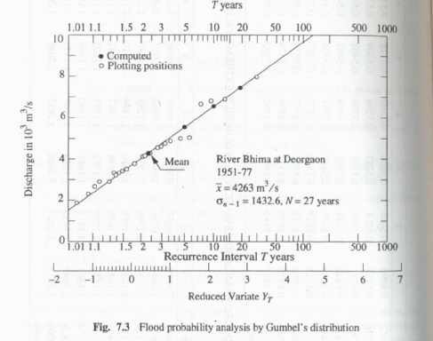
The  Gumbel  probability  paper  is  an  aid  for  convenient  graphical representation of Gumbel’ s distribution.

It consists of an abscissa specially marked for various  convenient values of the return period T. To construct the T scale on the abscjssa.

First construct an arithmetic scale of YT values, say from  —2 to + 7, as in Fig. 7.3. For selected values of T, say 2, 10, 50, 100,500 and 1000, find the values of YT by Equation (7.22) and mark off those positions on the abscissa. The T —scale is now ready for use (Fig. 7.3)

logarithmic scale. Since by Eqs (7.18) and (7.19) x varies linearly with yr, a Gumbel distribution will plot as a straight line on a Gumbel probability paper. This property can be used advantageously for graphical extrapolation, wherever necessary.

Other links:

HYDROLOGIC CYCLE
PRECIPITATION
RAIN GAUGE
EVAPORATION
INFILTRATION
GROUNDWATER
Water Table
AQUIFER PROPERTIES
DARCY’S LAW
FLOOD FREQUENCY STUDIES
RECURRENCE INTERVAL
FLOOD ROUTING

Categories
Uncategorized

RECURRENCE INTERVAL

RECURRENCE INTERVAL

RECURRENCE INTERVAL – In  many  hydraulic-engineering  applications  such  as  those  concerned  with floods, the probability of occurance  of  a  particular  extreme  rainfall,

e.g.  a  24-h maximum  rainfall,  will  be  of  importance.

Such  information  is  obtained  by  the frequency analysis of the point-rainfall data.

The rainfall at a place is a random hydrologic  process and the rainfall data at a place when arranged in chronological order constitute a time series.

One of the commonly used data series is the annual series composed of annual values such as annual rainfall.

If the extreme values of a specified event  occurring in each year is listed, it also constitutes an annual series.

Thus for example, one may list the maximum 24-h rainfall occurring in a year at  a  station  to  prepare  an  annual  series  of  24-h  maximum  rainfall  values.

The probability of occurrence of an event in this series is studied by frequency analysis of this annual data series.

A brief description of the terminology and a simple method of predicting the frequency of an event is described in this section and for details the reader  is referred  to standard  works  on  probability  and  statistics.

The  analysis  of annual series, even though described with rainfall as a reference is equally applicable to any other random hydrological process, e.g. stream flow.

First, it is necessary to correctly understand the terminology used in frequency analysis. The probability of occurrence of an event (e.g. rainfall) whose magnitude is equal to or in excess of a specified magnitude  X is denoted by P.

The recurrence interval (also known as return period) is defined as T=1/P

This represents the average interval between the occurrence of a rainfall of magnitude equal to or greater than X.

Thus if it is stated that the return period of rainfall of 20cm in  24  his  10  years  at  a  certain  station  A,  it  implies  that  on  an  average  rainfall magnitudes equal to or greater than 20 cm in 24 h occur once in 10 years, i.e. in a long period of say 100 years, 10 such events can be expected.

However, it does not mean that every 10 years one such event is likely, i.e. periodicity is not implied.

Then probability of a rainfall of 20 cm in 24 h occurring in any one year at station A is l/T = 1/10 = 0.1.

If the probability of an event occurring is P, the probability of the event not occurring in a given  year is q = ( 1- P).

The binomial distribution  can be used to find  the probability of occurrence of the event r times in n successive years. Thus

RECURRENCE INTERVAL

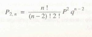
where Pr = probability of a random hydrologic event (rainfall) of given magnitude- and  exceedence  probability  P  occurring  r  times  in  n  successive  years.  Thus,  for example,

(a) The probability of an event  of exceedence probability P occurring 2 times inn successive years is

RECURRENCE INTERVAL

In  using  the  partial  duration  series,  it  is  necessary  to  establish  that  all  events considered are independent.

Hence the partial duration series is adopted mostly  for rainfall analysis where the  conditions of  independency of events are easy to establish its use in flood studies is rather.

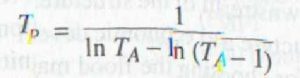
The recurrence interval of an event obtained by 100 series (TA) and by the Partial duration ( Tp) are related by

RECURRENCE INTERVAL

Other links:

HYDROLOGIC CYCLE
PRECIPITATION
RAIN GAUGE
EVAPORATION
INFILTRATION
GROUNDWATER
Water Table
AQUIFER PROPERTIES
DARCY’S LAW
FLOOD FREQUENCY STUDIES
GUMBEL’S METHOD
FLOOD ROUTING

Categories
Uncategorized

FLOOD – FLOOD FREQUENCY STUDIES

FLOOD

A flood is an unusually high stage in a river normally the level at which the river overflows its banks and inundates the adjoining area.

The damages caused by floods  in  terms  of  loss  of  life,  property  and  economic  loss  due  to  disruption  of economic activity are all too well known.

Crores of rupees are spent every year in flood control and flood forecasting.

The hydrograph of extreme floods and stages corresponding to flood peaks provide valuable data for purposes of hydrologic design.

Further, of the various characteristics of the flood hydrograph, probably the most important and widely used parameter is the flood peak.

At a given location in a stream, flood peaks vary from year to year and their magnitude constitutes a hydrologic series which enable one to assign  a  frequency  to  a  given  flood-peak  value.

In  the  design  of  practically  all hydraulic structures the peak flow that can be expected with an assigned frequency (say 1 in 100 years) is of primary importance to adequately proportion the structure to accommodate its effect.

The design of bridges, culvert waterways and spillways for dams and estimation of scour at a hydraulic  structure are some examples  wherein flood-peak values are required.

To estimate the magnitude of a flood peak the following alternative methods are available:

Rational method, empirical method, unit-hydrograph, and flood-frequency studies.

The use of a particular method depends upon (i) the desired objective, (ii) the available data and (iii) the importance of the project.

Further the rational formula is only applicable to small site (< 50 m) catchments and the unit-hydrograph method is normally restricted to moderate size catchments with areas less than 5000 km.

FLOOD FREQUENCY STUDIES

Hydrologic processes such as floods are exceedingly complex natural events.

They  are resultants  of a number  of component  parameters  and are  therefore  very difficult, analytically.

For example, the buds in a catchment depend upon the characteristics of the catchment, rainfall and antecedent conditions, each one of these factors in turn depend upon a host of constituent parameters.

This makes the elimination of the flood peak a very complex problem leading to many different approaches.

The empirical formulae and unit-hydrograph methods presented  in  the  previous  sections  are  some  of  them.  Another  approach  to  the prediction of flood flows, and also applicable to other hydrologic processes such as rainfall etc. is the statistical method of frequency analysis.

FLOOD FREQUENCY STUDIES

The values  of the maximum  flood  from a given  catchments  area for large number    of successive  years  constitute  a  hydrologic  data  series  called  the annual series.

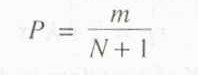
The  data  are  then  arranged  in  decreasing  order  of  magnitude  and  the probability  P  of  each  event  being  equaled  to  or  exceeded  (plotting  position)  is calculated by the plotting position formula

Where M = order number of the event and

N = total number of events in the data.

The recurrence  interval, T(also called the return period or frequency) is calculated as T=1/P

The last column shows the return period 1 of various flood magnitude, Q. A plot of Q vs T yields the probability distribution.

For small return periods (i.e. for interpolation) or where limited extrapolation is required, a simple best fitting curve through plotted points can be used as the probability distribution.

A logarithmic scale for T is often advantageous. However, when larger extrapolations of Tare  involved,  theoretical  probability  distributions  have  to  be  used.

In  frequency analysis of floods the usual problem is to predict extreme flood events. Towards this, specific  extreme-value  distributions  are assumed  and the required  statistical parameters calculated from the available data.

Using these  the flood magnitude for a specific return period is estimated.

Chow  (1951)  has shown that most  frequency  distribution functions applicable to hydrologic studies can be expressed by the following equation known as the general  equation of hydrologic frequency analysis:

where   x  = value of the variate X of a random hydrologic series with a return period T

x  = mean of the variate

= standard deviation of the variate

K = frequency  factor which depends upon the return period, T

and the assumed frequency  distribution.

Some of the commonly used frequency distribution function  predication of extreme flood values are

  • Gumbel’ s extreme —v alue distribution
  • Log —Pearson Type II distribution
  • Log normal distribution

Other links:

HYDROLOGIC CYCLE
PRECIPITATION
RAIN GAUGE
EVAPORATION
INFILTRATION
GROUNDWATER
Water Table
AQUIFER PROPERTIES
DARCY’S LAW
RECURRENCE INTERVAL
GUMBEL’S METHOD
FLOOD ROUTING

Categories
Uncategorized

DARCY’S LAW – Coefficient of Permeability

DARCY’S LAW

Darcy’s law – In 1856 Henry Darcy, a French hydraulic engineer, on the basis of his experimental findings proposed a law relating the velocity of flow in a porous medium. This law know as Darcy’s law can be expressed as

V = Ki

Where V= apparent velocity of discharge =Q/A Q= Discharge

A= Area of seepage medium

K  =  a  coefficient,  called  coefficient  of  permeability    having  the  units  of velocity.

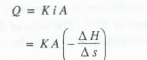
The discharge Q can be expressed as

DARCY’S LAW

Where –  H ( is the drop in the hydraulic  grade line in a length      s of the porous medium.

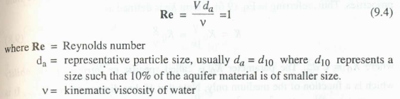
Darcy’s law is a particular case of the general viscous fluid flow. It has been valid for  laminar flows only. For practical purposes  the limit of the validity of Darcy’s law can be taken as Reynolds number of value unity, i.e.

DARCY’S LAW

Excepting for flow in fissures and caverns, to a large extent groundwater flow in  nature  obeys  Darcy’s  law.  Further,  there  is  no  known  lower  limit  for  the applicability of Darcy’s law.

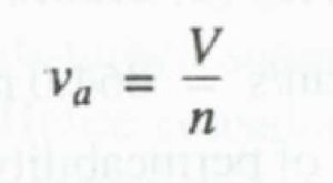
It may be noted that the apparent velocity V used in Darcy’s law is not the actual velocity of flow through the pores. Owing to irregular pore geometry the actual velocity of flow varies from point to point and the bulk pore velocity (Vs) which represents the actual speed of travel of water in the porous media is expressed as

where n = porosity. The bulk pore velocity v is the velocity that is obtained by tracking a tracer added to the groundwater.

Coefficient of Permeability

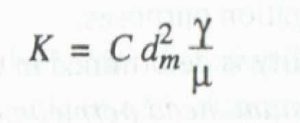
The  coefficient  of  permeability  also  designated  as  hydraulic  conductivity reflects the combined  effects of the porous medium and fluid properties.  From an analogy of laminar flow through a conduit (Hagen—P o iseuille flow) the coefficient of Permeability can be expressed as

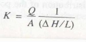
The coefficient of permeability is determined in the laboratory by a permeameter . For coarse grained  soils a constant  head permeability  is used. In this the discharge  of water percolating under a constant head difference ( H) through a sample, of porous material of cross. area A and length l is determined. The coefficient of permeability at the temperature of the experiment is found as

For fine grained soils, falling head permeameter is used. It should be noted that laboratory samples are disturbed samples and a permeameter cannot simulate the field conditions exactly. Hence considerable care in the preparation of the samples and in conducting the tests are needed to obtain meaningful results.

Under  field  conditions,  permeability  of  an  aquifer  is  determined  by  conducting pumping tests in a well. One of the many tests available for this purpose consists of pumping out water from a well at a uniform rate till steady state is reached. Knowing the steady state drawdown and the discharge rate, transmissibility can be calculated. Information   about the thickness of the saturation zone leads one to calculate the Permeability. Injection of a tracer, such as a dye and finding its velocity of travel is another way of determining the permeability under field conditions.

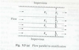
Sometimes the aquifers may be stratified, with different permeabilities in each-strata. T kinds of flow situations are possible in such a case.

(i)  When  the  flow  is  parallel  to  the  stratification  as  in  Fig.  9.5  (a)  equivalent

Permeability Ke of the entire aquifer of thickness

Other links:

HYDROLOGIC CYCLE
PRECIPITATION
RAIN GAUGE
EVAPORATION
INFILTRATION
GROUNDWATER
Water Table
AQUIFER PROPERTIES
FLOOD FREQUENCY STUDIES
RECURRENCE INTERVAL
GUMBEL’S METHOD
FLOOD ROUTING

Categories
Uncategorized

Water Table, AQUIFER PROPERTIES

Water Table

A water table is the free water surface in an unconfined  aquifer. The static level of a well penetrating  an unconfirmed  aquifer indicates the level of the water table at that point.

The water table is constantly in motion adjusting its surface  to achieve a balance between the recharge and outflow from the subsurface storage.

Fluctuations  in the  water level in a dug  well during  various  seasons  of the  year, lowering of the groundwater table in a region due to heavy pumping of the wells and the rise in the water table of an irrigated area with poor drainage, are some common examples of the fluctuation of the water table.

In a general sense, the water table follows the topographic features of the surface.

In the water table intersects the land surface the groundwater comes out to the surface in the form of springs or seepage.

Sometimes a lens or localized patch of impervious stratum can occur inside an unconfined aquifer in such a way that it retains a water table above the general water table (Fig. 9.3).

Such a water table retained around the impervious material is known as perched water table. Usually the perched water table is of limited extent and the yield from such a situation is very small. In groundwater exploration a perched water table is quite often confused with a general water table.

The  position  of  the  water table  relative  to  the  water  level  in  a  stream determines  whether the stream contributes  water to the groundwater  storage or the other way about.

If the bed of the  stream  is below the groundwater  table, during periods of low flows in the stream, the water surface may go down below the general water table elevation and the groundwater contributes to the flow in the stream.

Such streams which receive groundwater flow are called effluent streams (Fig. 9.4 (a)).

water table

Perennial rivers and streams are of this kind. If, however, the water table is below the bed of the stream, the stream-water percolates to the groundwater storage and a hump is formed in the groundwater table (Fig. 9.4 (h)).

Such streams which contribute to the groundwater are knows as influent streams. Intermittent rivers and streams which go dry during long periods of dry spell (i.e. no rain periods) are of this kind.

AQUIFER PROPERTIES

The important properties of an aquifer are its capacity to release the water held in its pores and its ability to transmit the flow easily.

These properties  essentially depend upon the composition of the aquifer.

Porosity

The amount of pore space per unit volume of the aquifer material is called porosity. It is expressed

Specific Yield

While porosity gives a measure of the water storage capability of a formation C the water held in the pores is available for extraction by Pumping or draining by gravity.

The poles hold back some water by molecular  attraction and surface  tension.

The actual volume of water that can be extracted by the force of gravity from a unit of aquifer material is known as the Specific yield Sy.

The fraction of a unit held back in the aquifer is known as specific retention.

Thus Porosity of water

Other links:

HYDROLOGIC CYCLE
PRECIPITATION
RAIN GAUGE
EVAPORATION
INFILTRATION
GROUNDWATER
DARCY’S LAW
FLOOD FREQUENCY STUDIES
RECURRENCE INTERVAL
GUMBEL’S METHOD
FLOOD ROUTING

Categories
Uncategorized

groundwater

GROUNDWATER

Study  of  subsurface  flow  is  equally important since about 30% of the world’s fresh water resources exist in the form of groundwater.

Further, the subsurface water forms a critical input for the sustenance of life and vegetation in arid zones.

Because of its importance as a significant source of water   supply,   various   aspects   of   groundwater   dealing   with   the   exploration, development and utilization have been extensively studied by workers from different disciplines, such as geology, geophysics, geochemistry, agricultural engineering, fluid mechanics and civil engineering and excellent treatises are available.

FORMS OF SUBSURFACE WATER

Water in the soil mantle is called subsurface water and is considered in two zones (Fig. 9.1):

Saturated zone aeration zone

groundwater

Saturated Zone

This zone, also known as groundwater zone, is the space in which all the pores of the soil are filled with water.

The water table forms its upper limit and marks a free surface, i.e. a surface having atmospheric pressure.

Zone of Aeration

In this zone the soil pores are only partially saturated with water.

The space between the land surface and the water table marks the extent of this zone.

Further, the zone of aeration has three subzones:

Soil Water Zone

This lies close to the ground surface in the major root band of the vegetation from which the water is lost to the atmosphere by evapotranspiration.

Capillary Fringe

In this the water is held by capillary action.

This zone extends from the water table upwards to the limit of the capillary rise.

Intermediate Zone

This lies between the soil water zone and the capillary fringe.

The thickness of the zone of aeration and its constituent subzones depend upon the  soil  texture  and  moisture  content  and  vary  from  region  to  region.

The  soil moisture in the zone of aeration is of importance in agricultural practice and irrigation engineering.

The present chapter is concerned only with the saturated zone.

All earth materials, from soils to rocks have pore spaces. Although these pores are completely saturated with water below the water table, from the groundwater utilization aspect only such material through which water moves easily and hence can be  extracted  with  ease  are  significant.

On  this basis  the  saturated  formations  are classified into four categories

�   Aquifer

�   Aquitard

�   Aquiclude

�   Aquifuge

These are discussed below:

Aquifer

An aquifer is a saturated  formation of earth material which not only stores water but yields it in sufficient quantity.

Thus an aquifer transmits water relatively easily due to its high permeability. Unconsolidated deposits of sand and gravel form good aquifers.

Aquitard

It is a formation through which only seepage is possible and thus the yield is insignificant compared to an aquifer. It is partly permeable.

A sandy clay unit is an example of aquitard. Through an aquitard appreciable quantities of water may leak to an aquifer below it.

Aquiclude

it is a geological formation which is essentially impermeable  to the flow of water.

It may be considered as closed to water movement even though it may contain large amounts of water due to its high porosity. Clay is an example of an aquiclude.

Aquifuge

It is a geological formation which is neither porous nor permeable. There are no interconnected openings and hence it cannot transmit water. Massive compact rock without any fractures is an aquifuge.

The definitions of aquifer, aquitard and aquiclude as above are relative.

A formation  which  may be considered  as an aquifer  at a place  where  water  is at a premium (e.g. arid zohes) may be classified as an aquitard or even aquiclude in an area where plenty of water is available.

The availability of groundwater from an aquifer at a place depends upon the rates of withdrawal and replenishment  (recharge).

Aquifers play the roles of both a transmission conduit and a storage.

Aquifers are classified as unconfined aquifers and confined aquifers on the basis of their occurrence and field situation.

An unconfined aquifer (also known as water table aquifer) is one in which a free water surface, i.e. a water table exists (Fig. 9.2).

Only the saturated zone of this aquifer is of importance in groundwater studies.

Recharge of this aquifer takes place through infiltration of precipitation from the ground surface.

A well driven into an unconfined aquifer will indicate a static water level corresponding to the water table level at that location.

A confined aquifer, also known as artesian aquifer, is an aquifer which is confined between two impervious beds such as aquicludes or aquifuges (Fig. 9.2).

Recharge of this aquifer takes place only in the area where it is exposed at the ground surface.

The water in the confined aquifer will be under pressure and hence the piezometric level will be much higher than the top level of the aquifer.

At some locations: the piezoelectric  level can attain a level higher than the land  surface  and a well driven  into the aquifer at such a location will flow freely without the aid of any pump.

In fact, the term “artesian” is derived from the fact that a large number of such free flow wells were found in Artois, a former province in north France.

Instances of free-flowing wells having as much as a 50-rn head at  the ground surface are reported.

A confined aquifer is called a leaky aquifer if either or both of its confining beds are aquitards.

groundwater

Other links:

HYDROLOGIC CYCLE
PRECIPITATION
RAIN GAUGE
EVAPORATION
INFILTRATION
Water Table
AQUIFER PROPERTIES
DARCY’S LAW
FLOOD FREQUENCY STUDIES
RECURRENCE INTERVAL
GUMBEL’S METHOD
FLOOD ROUTING

Categories
Uncategorized

INFILTRATION

INFILTRATION

INFILTRATION is well-known that when water is applied to the surface of a soil, a part of it seeps into the soil.

This movement of water through the soil surface is known as illustration and plays a very significant role in the runoff process by affecting the timing distribution and magnitude of the surface runoff.

Further, infiltration is the prim step in the natural groundwater recharge.

Infiltration is the flow of water into the go through the soil surface and the process can be easily understood through a simple analogy.

Consider a small container covered with wire gauze a$ in Fig. 3.8. If water is poured over the gauze, a part of it will go into the container and a part overflow.

Further, the container can hold only a fixed quantity and when it is full no more flow into the contain can take place.

This analogy, though a highly simplified one, underscores two important aspects, viz., (1) the maximum rate at which the ground can absorb water, the infiltration capacity and (ii) the volume of water that it can hold, the field capacity.

INFILTRATION CAPACITY

The maximum rate -at which a given soil at a given time can absorb water is defined as the infiltration capacity.

It is designated as the infiltration f and is expressed in units of cm/h.

where i = intensity of rainfall.

The infiltration capacity of a soil is high at the beginning  of  a  storm  and  has  an  exponential  decay  as  the  time  elapses.

The infiltration process is affected by a large number of factors and a few important ones affecting are described below.

Characteristics of Soil

The type of soil, viz, sand, silt or clay, its texture, structure, permeability and under drainage are the important characteristics under this category.

A loose, permeable, sandy soil will have a larger infiltration capacity than a tight, clayey soil.

A soil with good under drainage, i.e. the facility to transmit the infiltered water downward to a groundwater storage would obviously have a higher infiltration capacity.

When the soils occur in layers, the transmission capacity of the layers determine the overall infiltration rate.

Also, a dry soil can absorb more water than one whose pores are already full.

The land use has a significant influence on fc For example, a forest soil rich in organic matter will have a much higher value of ft under identical conditions than the same soil in an urban area where it is subjected to compaction.

Surface of Entry

At the soil surface, the impact of raindrops causes the fines in the soils to be displaced and these in turn can clog the pore spaces in the upper layers. This is an important factor affecting the infiltration capacity. Thus a surface covered by grass and other Vegetation which can reduce this process has a pronounced influence on the value of

Fluid Characteristics

Water infiltrating into the soil will have many impurities, both in solution and in suspension. The turbidity of the water, especially the clay and colloid content is an important factor as such suspended particles block the fine pores in the soil and reduce its infiltration capacity.

The temperature of the water is a factor in the sense that it affects the viscosity of the water which in turn affects the infiltration rate. Contamination of the water by dissolved salts can affect the soil structure and in turn affect the infiltration rate.

MEASUREMENT OF INFILTRATION

Information about the infiltration characteristics of the soil at a given location can be obtained by conducting controlled experiments on small areas. The experimental set- up is called an infiltrometer.

There are two kinds of infiltrometers:

Flooding-type infiltrometer

Rainfall simulator.

Flooding-Type Infiltrometer:

This is a simple instrument consisting essentially of a metal cylinder, 30cm diameter and 60cm long, open at both ends.

This cylinder is driven into the ground to a depth of 50cm (Fig. 3.10). Water is poured into the top part to a depth of 5cm and a pointer is set to mark the water level.

As infiltration proceeds, the volume is made up by adding water from a burette to keep the water level at the tip of the pointer.

Knowing the volume of water added at different time intervals, the plot of the infiltration capacity vs time is obtained.

The experiments are continued fill a uniform rate of infiltration is obtained and this may take 2-3 h.

The surface of the soil is usually protected by a perforated disk to prevent formation of turbidity and its settling on the soil surface.

A major objection to the simple infiltrometer as above is that the infiltered water spreads at the outlet from the tube (as shown by dotted lines in Fig. 3.10) and as such the tube area is not representative of the area in which infiltration takes place.

To overcome this a ring infiltrometer consisting of a set of two concentric rings (Fig 3.11) is used. In this two rings as inserted into the ground and water is maintained on the soil surface, in both the rings, to a common fixed level.

The outer ring provides a water jacket to the filtering water of the inner ring and hence prevents the spreading out of the f water of the inner tube. The measurements of water volume is done on the inner ring only.

Disadvantages of flooding-type infiltrometers:

1.The raindrop-impact effect is not simulated

2. The driving of the tube or rings disturbs the soil structure

3. The results of the infiltrometer depend to some extent on their size with the larger meters giving less rates than the smaller ones; this is due to the border effect.

Rainfall Simulator

In this a small plot of land, of about 2 m x 4 m size, is provided with a series of nozzles on the longer side with arrangements to collect and  measure the surface runoff rate.

The specially designed nozzles produce raindrops falling from a height of 2 in and are capable of producing various intensities of rainfall.

Experiments are conducted under controlled conditions with various combinations of intensities and durations and the surface runoff is measured in each case.

Using the water-budget equation involving the volume of rainfall, infiltration and runoff, the infiltration rate and its variation with time are calculated.

If the rainfall intensity is higher than the infiltration rate, infiltration-capacity values are obtained. Rainfall simulator type infiltrometers given lower values than flooding­ type infiltrometers.

This is due to the effect of the rainfall impact and turbidity of the surface water present in the former.

Other links:

HYDROLOGIC CYCLE
PRECIPITATION
RAIN GAUGE
EVAPORATION
GROUNDWATER
Water Table
AQUIFER PROPERTIES
DARCY’S LAW
FLOOD FREQUENCY STUDIES
RECURRENCE INTERVAL
GUMBEL’S METHOD
FLOOD ROUTING